Bank Transaction Fraud Detection 01

Problem Statement

With the rapid growth of digital banking, fraudulent transactions have become a significant concern for financial institutions. The challenge is to build a robust system to detect and prevent fraudulent transactions in real-time while maintaining customer convenience and privacy.

The dataset provided contains detailed information about bank transactions, including customer demographics, transaction metadata, merchant categories, device types, transaction locations, and other relevant attributes. Key fields like transaction descriptions, device usage, and merchant categories provide vital insights for identifying anomalous activities. The "Is_Fraud" label offers a foundation for supervised learning techniques to differentiate between genuine and fraudulent transactions.

The objective of this problem is to analyze transaction patterns and develop predictive models that can accurately classify transactions as fraudulent or legitimate. This task involves exploring feature correlations, detecting unusual transaction behavior, and leveraging machine learning algorithms to create a scalable and efficient fraud detection system.

A successful solution will not only detect fraudulent activities but also minimize false positives, ensuring genuine transactions are not unnecessarily flagged. Insights derived from this analysis can help strengthen security measures, optimize fraud prevention strategies, and enhance the overall banking experience for customers.

Objectives for Bank Transaction Fraud Detection

Fraud Detection:
- Develop a predictive model to classify bank transactions as fraudulent or legitimate using historical transaction data.
Anomaly Detection:
- Identify unusual patterns or behaviors in customer transactions that may indicate potential fraud.
Feature Analysis:
- Explore key features such as merchant categories, transaction devices, transaction locations, and account types to understand their impact on fraud detection.
Model Performance Optimization:
- Ensure the fraud detection system achieves high accuracy, precision, and recall while minimizing false positives and false negatives.
Real-Time Fraud Prevention:
- Create a scalable solution that can potentially be adapted for real-time fraud detection in production environments.
Customer Behavior Insights:
- Analyze legitimate transaction behaviors to gain insights into customer banking patterns and preferences.
Device and Location Security:
- Understand the correlation between transaction device types, locations, and fraudulent activities.
Security Enhancements:
- Provide actionable recommendations to the bank for improving fraud prevention strategies and enhancing digital transaction security.

Technologies Used

Python
Scikit-learn
Pandas
NumPy

Jupyter Notebook

Stage 1 - Importing Libraries

# Import necessary libraries
import pandas as pd
import numpy as np
import matplotlib.pyplot as plt
import seaborn as sns
from imblearn.over_sampling import SMOTE
from sklearn.decomposition import PCA
from sklearn.utils.class_weight import compute_class_weight
from sklearn.neighbors import KNeighborsClassifier
from sklearn.naive_bayes import GaussianNB
from sklearn.model_selection import train_test_split, cross_val_score, GridSearchCV
from sklearn.preprocessing import StandardScaler, LabelEncoder
from sklearn.metrics import classification_report, confusion_matrix, roc_auc_score
from sklearn.linear_model import LogisticRegression
# from sklearn.linear_model import LinearDiscriminantAnalysis as LDA, RidgeClassifier
from sklearn.tree import DecisionTreeClassifier
from sklearn.ensemble import RandomForestClassifier, GradientBoostingClassifier, AdaBoostClassifier, BaggingClassifier
from sklearn.svm import SVC, LinearSVC
from sklearn.metrics import accuracy_score, classification_report, confusion_matrix
from sklearn import metrics
import xgboost as xgb
import lightgbm as lgb
import catboost as cb
import warnings

# Suppress all warnings
warnings.filterwarnings("ignore")

# Load the dataset
df = pd.read_csv('Bank_Transaction_Fraud_Detection.csv')
df.head()

Output

 	Customer_ID 	                        Customer_Name 	      Gender 	Age 	State 	        City 	             Bank_Branch                   Account_Type     Transaction_ID 	                        Transaction_Date 	... 	Merchant_Category   Account_Balance 	Transaction_Device    Transaction_Location             Device_Type   Is_Fraud 	Transaction_Currency 	Customer_Contact    Transaction_Description    Customer_Email
d5f6ec07-d69e-4f47-b9b4-7c58ff17c19e 	Osha Tella            Male      60      Kerala 	        Thiruvananthapuram   Thiruvananthapuram Branch     Savings          4fa3208f-9e23-42dc-b330-844829d0c12c 	23-01-2025 	        ... 	Restaurant          74557.27 	        Voice Assistant       Thiruvananthapuram, Kerala       POS           0 	        INR 	                +9198579XXXXXX 	    Bitcoin transaction        oshaXXXXX@XXXXX.com
7c14ad51-781a-4db9-b7bd-67439c175262 	Hredhaan Khosla       Female    51      Maharashtra 	Nashik               Nashik Branch                 Business         c9de0c06-2c4c-40a9-97ed-3c7b8f97c79c 	11-01-2025 	        ... 	Restaurant          74622.66 	        POS Mobile Device     Nashik, Maharashtra              Desktop       0 	        INR 	                +9191074XXXXXX 	    Grocery delivery           hredhaanXXXX@XXXXXX.com
3a73a0e5-d4da-45aa-85f3-528413900a35 	Ekani Nazareth 	      Male      20      Bihar 	        Bhagalpur            Bhagalpur Branch              Savings          e41c55f9-c016-4ff3-872b-cae72467c75c 	25-01-2025 	        ... 	Groceries           66817.99 	        ATM                   Bhagalpur, Bihar                 Desktop       0 	        INR 	                +9197745XXXXXX 	    Mutual fund investment     ekaniXXX@XXXXXX.com
7902f4ef-9050-4a79-857d-9c2ea3181940 	Yamini Ramachandran   Female    57      Tamil Nadu      Chennai              Chennai Branch                Business         7f7ee11b-ff2c-45a3-802a-49bc47c02ecb 	19-01-2025 	        ... 	Entertainment       58177.08 	        POS Mobile App        Chennai, Tamil Nadu              Mobile        0 	        INR 	                +9195889XXXXXX 	    Food delivery              yaminiXXXXX@XXXXXXX.com
3a4bba70-d9a9-4c5f-8b92-1735fd8c19e9 	Kritika Rege 	      Female    43      Punjab 	        Amritsar             Amritsar Branch               Savings          f8e6ac6f-81a1-4985-bf12-f60967d852ef 	30-01-2025 	        ... 	Entertainment       16108.56 	        Virtual Card          Amritsar, Punjab                 Mobile        0 	        INR 	                +9195316XXXXXX 	    Debt repayment             kritikaXXXX@XXXXXX.com

df.info()

Output

df.shape

Output

(200000, 24)

df.duplicated().sum()

Output

Stage 2 - Data Preprocessing

# Checking for missing values
print("Missing NULL values in the dataset:")
print(df.isnull().sum())
print("-"*80)
print("Missing N/A values in the dataset:")
print(df.isna().sum())

Output

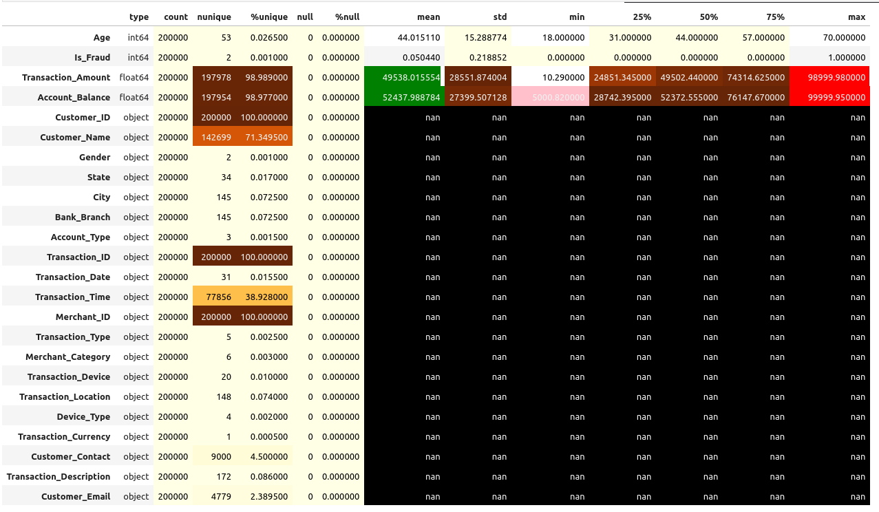
desc = pd.DataFrame(index = list(df))
desc['type'] = df.dtypes
desc['count'] = df.count()
desc['nunique'] = df.nunique()
desc['%unique'] = desc['nunique'] /len(df) * 100
desc['null'] = df.isnull().sum()
desc['%null'] = desc['null'] / len(df) * 100
desc = pd.concat([desc,df.describe().T.drop('count',axis=1)],axis=1)
desc.sort_values(by=['type','null']).style.background_gradient(cmap='YlOrBr')\
    .bar(subset=['mean'],color='green')\
    .bar(subset=['max'],color='red')\
    .bar(subset=['min'], color='pink')

Output

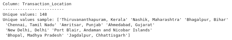
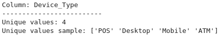
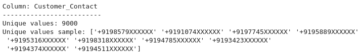
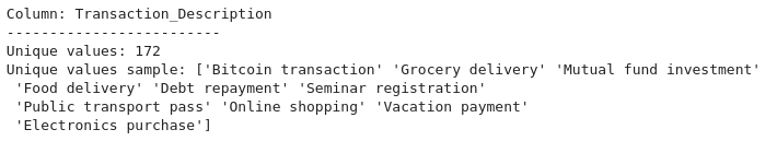
# Get a list of categorical columns in the dataframe
categorical_columns = df.select_dtypes(include=['object']).columns

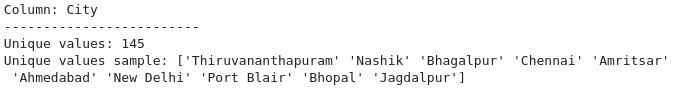
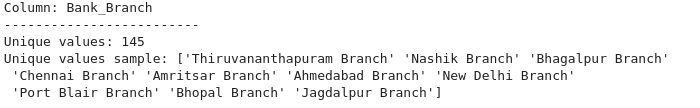
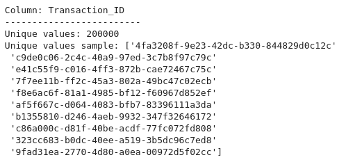
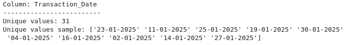
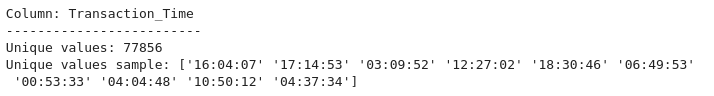
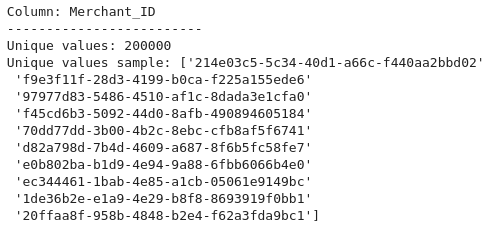
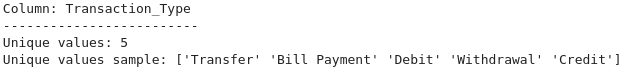
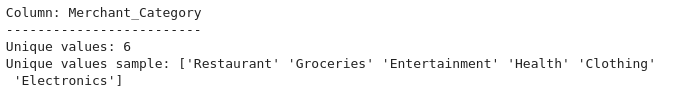
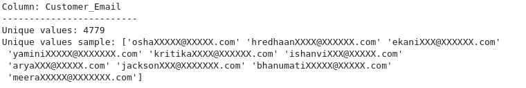
# Check the unique values and their counts for each categorical column
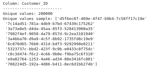
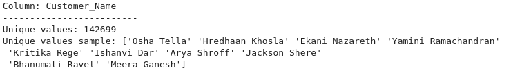
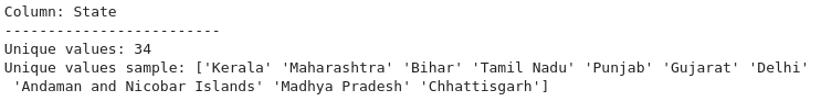
for col in categorical_columns:
    print(f"Column: {col}")
    print("-" * 25)
    print(f"Unique values: {df[col].nunique()}")
    print(f"Unique values sample: {df[col].unique()[:10]}")  # Display a sample of unique values
    print("-" * 50)

Output

Check the unique values and their counts for each categorical column

# If a column has only one unique value, it won't be useful for prediction.
single_value_columns = [col for col in df.columns if df[col].nunique() == 1]
print("Columns with only one unique value:", single_value_columns)

# Dropping columns with one unique value
df = df.drop(columns=single_value_columns)

Output

Columns with only one unique value: ['Transaction_Currency']

# Checking columns after dropping one unique columns
df.columns

Output

Index(['Customer_ID', 'Customer_Name', 'Gender', 'Age', 'State', 'City',
       'Bank_Branch', 'Account_Type', 'Transaction_ID', 'Transaction_Date',
       'Transaction_Time', 'Transaction_Amount', 'Merchant_ID',
       'Transaction_Type', 'Merchant_Category', 'Account_Balance',
       'Transaction_Device', 'Transaction_Location', 'Device_Type', 'Is_Fraud',
       'Customer_Contact', 'Transaction_Description', 'Customer_Email'],
      dtype='object')

# Drop the columns which are not useful for the model evaluation
df = df.drop(columns=['Customer_Contact', 'Customer_Email', 'Customer_Name', 'Customer_ID', 'Transaction_ID', 'Merchant_ID'])
print(df.shape)

Output

(200000, 17)

# Checking columns after dropping not useful columns
df.columns

Output

Index(['Gender', 'Age', 'State', 'City', 'Bank_Branch', 'Account_Type',
       'Transaction_Date', 'Transaction_Time', 'Transaction_Amount',
       'Transaction_Type', 'Merchant_Category', 'Account_Balance',
       'Transaction_Device', 'Transaction_Location', 'Device_Type', 'Is_Fraud',
       'Transaction_Description'],
      dtype='object')

Stage 3 - Exploratory Data Analysis (EDA)

EDA for Numerical Columns

# For numerical columns, we'll fill missing values with the median of each column
numerical_columns = df.select_dtypes(include=['float64', 'int64']).columns
for col in numerical_columns:
    df[col] = df[col].fillna(df[col].median())

print(numerical_columns)

Output

Index(['Age', 'Transaction_Amount', 'Account_Balance', 'Is_Fraud'], dtype='object')

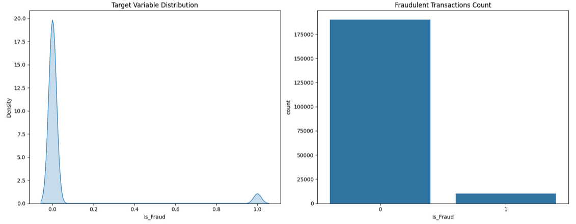
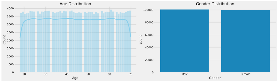
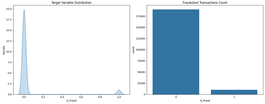
# Create a figure with 2 subplots in a horizontal row
fig, axes = plt.subplots(1, 2, figsize=(15, 6))  # 1 row, 2 columns

# KDE plot for the 'Is_Fraud' column (on the first subplot)
sns.kdeplot(df["Is_Fraud"], fill=True, ax=axes[0])
axes[0].set_title('Target Variable Distribution')

# Count plot for the 'Is_Fraud' column (on the second subplot)
sns.countplot(x='Is_Fraud', data=df, ax=axes[1])
axes[1].set_title('Fraudulent Transactions Count')

# Adjust layout to prevent overlap
plt.tight_layout()

# Show the plot
plt.show()

Output

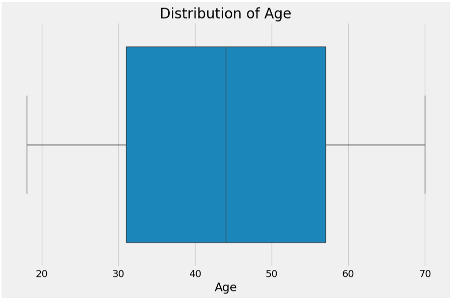
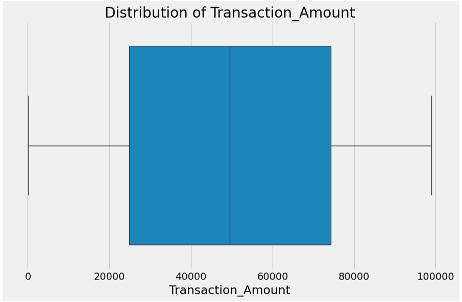
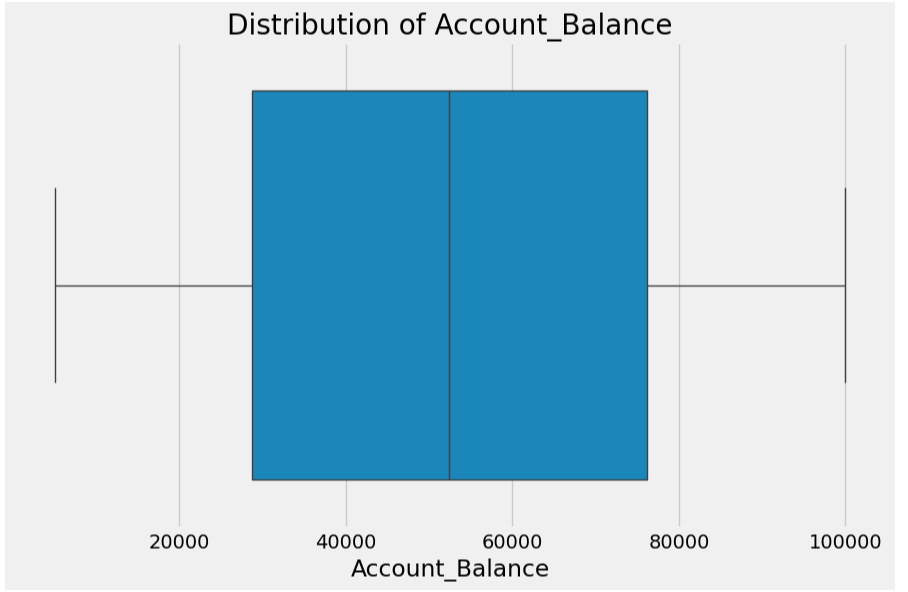
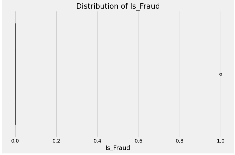
# Loop through each numerical column in your DataFrame
for col in numerical_columns:
    plt.style.use("fivethirtyeight")
    plt.figure(figsize=(10, 6))

    # Create the boxplot
    sns.boxplot(x=df[col])
    plt.title(f'Distribution of {col}')
    plt.xlabel(col)

    # Show the plot
    plt.show()

Output

EDA for Categorical Columns

Index(['Customer_ID', 'Customer_Name', 'Gender', 'State', 'City',
       'Bank_Branch', 'Account_Type', 'Transaction_ID', 'Transaction_Date',
       'Transaction_Time', 'Merchant_ID', 'Transaction_Type',
       'Merchant_Category', 'Transaction_Device', 'Transaction_Location',
       'Device_Type', 'Transaction_Currency', 'Customer_Contact',
       'Transaction_Description', 'Customer_Email'],
      dtype='object')

Output

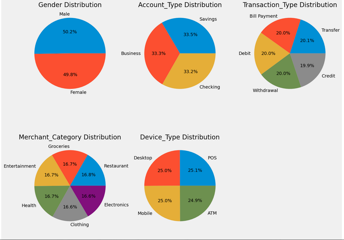
# Calculate the number of rows needed based on the number of charts
num_cols = 3  # Number of charts per row
# num_rows = (len(categorical_columns) + num_cols - 1) // num_cols  # Calculate rows required for all charts
num_rows = 2 # Number of rows
fig, axes = plt.subplots(num_rows, num_cols, figsize=(15, num_rows * 6))  # Adjust figure size for more rows

# Flatten the axes array for easier iteration
axes = axes.flatten()

ax_index = 0
for col in categorical_columns:
    unique_values = df[col].nunique()
    if unique_values < 10:  # Only plot if unique values are less than 10
        # Plot on the respective subplot
        ax = axes[ax_index]
        ax.pie(df[col].value_counts(), labels=df[col].unique(), autopct='%1.1f%%')
        ax.set_title(f'{col} Distribution')

        # Move to the next subplot
        ax_index += 1

# Hide any unused subplots (in case there are fewer than `num_rows * num_cols` charts)
for i in range(ax_index, len(axes)):
    axes[i].axis('off')

# Adjust layout
plt.tight_layout()
plt.show()

Output

import matplotlib.pyplot as plt
import seaborn as sns

# Filter categorical columns with less than 20 unique values
categorical_cols = df.select_dtypes(include=['object']).columns
categorical_cols = [col for col in categorical_cols if df[col].nunique() < 20]

# Set the number of charts per row and rows
num_cols = 3  # Number of charts per row
num_rows = 2  # Number of rows

# Calculate the total number of subplots needed
total_plots = len(categorical_cols)

# Create a figure with the appropriate number of rows and columns
plt.figure(figsize=(15, 5 * num_rows))

# Plot the count plots for the filtered categorical columns
for i, col in enumerate(categorical_cols):
    plt.subplot(num_rows, num_cols, i + 1)
    sns.countplot(data=df, x=col, hue='Is_Fraud')
    plt.title(f'Fraud by {col}')
    plt.xticks(rotation=45)

plt.tight_layout()
plt.show()

# Calculate churn rate by categories
print("\Fraud Rate by Categories:")
for col in categorical_cols:
    print(f"\n{col} Analysis:")
    print(df.groupby(col)['Is_Fraud'].mean().round(3) * 100)

Output

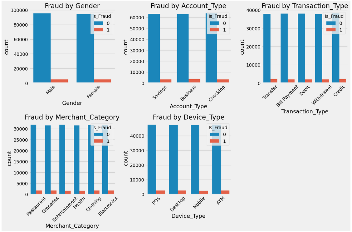
\Fraud Rate by Categories:

Gender Analysis:
Gender
Female    5.0
Male      5.1
Name: Is_Fraud, dtype: float64

Account_Type Analysis:
Account_Type
Business    5.2
Checking    4.9
Savings     5.0
Name: Is_Fraud, dtype: float64

Transaction_Type Analysis:
Transaction_Type
Bill Payment    4.9
Credit          5.1
Debit           5.1
Transfer        5.2
Withdrawal      4.9
Name: Is_Fraud, dtype: float64

Merchant_Category Analysis:
Merchant_Category
Clothing         5.2
Electronics      5.0
Entertainment    4.8
Groceries        5.2
Health           5.0
Restaurant       5.0
Name: Is_Fraud, dtype: float64

Device_Type Analysis:
Device_Type
ATM        5.0
Desktop    5.1
Mobile     5.0
POS        5.1
Name: Is_Fraud, dtype: float64

Stage 4 - Convert Date Time Columns to Numerical Columns

Convert 'Transaction_Date' and 'Transaction_Time' to datetime

df['Transaction_Date'] = pd.to_datetime(df['Transaction_Date'], format='%d-%m-%Y')
df['Transaction_Time'] = pd.to_datetime(df['Transaction_Time'], format='%H:%M:%S')

# Extract new features from 'Transaction_Date' and 'Transaction_Time'
df['Transaction_Day'] = df['Transaction_Date'].dt.day
df['Transaction_Month'] = df['Transaction_Date'].dt.month
df['Transaction_Year'] = df['Transaction_Date'].dt.year
df['Transaction_Hour'] = df['Transaction_Time'].dt.hour
df['Transaction_Minute'] = df['Transaction_Time'].dt.minute
df['Transaction_Second'] = df['Transaction_Time'].dt.second

# Drop 'Transaction_Date' and 'Transaction_Time' columns after feature extraction
df = df.drop(columns=['Transaction_Date', 'Transaction_Time'])

# If a column has only one unique value, it won't be useful for prediction.
single_value_cols = [col for col in df.columns if df[col].nunique() == 1]
print("Columns with only one unique value:", single_value_columns)

# Dropping columns with one unique value
df = df.drop(columns=single_value_cols)

Output

Columns with only one unique value: ['Transaction_Currency']

# For numerical columns, updating after conversion
numerical_columns = df.select_dtypes(include=['float64', 'int64']).columns
print("Numerical Columns ::", numerical_columns)
print("-"*50)
# For categorical columns, updating after conversion
categorical_columns = df.select_dtypes(include=['object']).columns
print("Categorical Columns ::", categorical_columns)

Output

Numerical Columns :: Index(['Age', 'Transaction_Amount', 'Account_Balance', 'Is_Fraud'], dtype='object')
--------------------------------------------------
Categorical Columns :: Index(['Gender', 'State', 'City', 'Bank_Branch', 'Account_Type',
       'Transaction_Type', 'Merchant_Category', 'Transaction_Device',
       'Transaction_Location', 'Device_Type', 'Transaction_Description'],
      dtype='object')

df.head()

Output

 	Gender 	Age 	State        City                 Bank_Branch                   Account_Type 	Transaction_Amount  Transaction_Type    Merchant_Category    Account_Balance   Transaction_Device   Transaction_Location        Device_Type 	Is_Fraud    Transaction_Description   Transaction_Day   Transaction_Hour   Transaction_Minute   Transaction_Second
Male 	60      Kerala       Thiruvananthapuram   Thiruvananthapuram Branch     Savings         32415.45            Transfer            Restaurant           74557.27          Voice Assistant      Thiruvananthapuram, Kerala  POS             0           Bitcoin transaction       23                16                 4                     7
Female 	51      Maharashtra  Nashik 	          Nashik Branch                 Business        43622.60            Bill Payment        Restaurant           74622.66          POS Mobile Device    Nashik, Maharashtra         Desktop         0           Grocery delivery          11                17                 14                    53
Male 	20      Bihar        Bhagalpur            Bhagalpur Branch              Savings         63062.56            Bill Payment        Groceries            66817.99          ATM                  Bhagalpur, Bihar            Desktop         0           Mutual fund investment    25                3                  9                     52
Female 	57      Tamil Nadu   Chennai              Chennai Branch                Business        14000.72            Debit               Entertainment        58177.08          POS Mobile App       Chennai, Tamil Nadu         Mobile          0           Food delivery             19                12                 27                    2
Female 	43      Punjab       Amritsar             Amritsar Branch               Savings         18335.16            Transfer            Entertainment        16108.56          Virtual Card         Amritsar, Punjab            Mobile          0           Debt repayment            30                18                 30                    46

Stage 5 - Encode Categorical Features

# Initializing the LabelEncoder
label_encoder = LabelEncoder()

for col in categorical_columns:
    df[col] = label_encoder.fit_transform(df[col])

df.head()

Output

 	Customer_ID                             Customer_Name       Gender 	Age    State        City                 Bank_Branch                 Account_Type   Transaction_ID                          Transaction_Date   ...   Merchant_Category   Account_Balance   Transaction_Device   Transaction_Location          Device_Type   Is_Fraud   Transaction_Currency   Customer_Contact   Transaction_Description   Customer_Email
d5f6ec07-d69e-4f47-b9b4-7c58ff17c19e    Osha Tella          Male 	60     Kerala       Thiruvananthapuram   Thiruvananthapuram Branch   Savings        4fa3208f-9e23-42dc-b330-844829d0c12c    23-01-2025         ...   Restaurant          74557.27          Voice Assistant      Thiruvananthapuram, Kerala    POS           0          INR                    +9198579XXXXXX     Bitcoin transaction       oshaXXXXX@XXXXX.com
7c14ad51-781a-4db9-b7bd-67439c175262    Hredhaan Khosla     Female 	51     Maharashtra  Nashik               Nashik Branch               Business       c9de0c06-2c4c-40a9-97ed-3c7b8f97c79c    11-01-2025         ...   Restaurant          74622.66          POS Mobile Device    Nashik, Maharashtra           Desktop       0          INR                    +9191074XXXXXX     Grocery delivery          hredhaanXXXX@XXXXXX.com
3a73a0e5-d4da-45aa-85f3-528413900a35    Ekani Nazareth      Male 	20     Bihar        Bhagalpur            Bhagalpur Branch            Savings        e41c55f9-c016-4ff3-872b-cae72467c75c    25-01-2025         ...   Groceries           66817.99          ATM                  Bhagalpur, Bihar              Desktop       0          INR                    +9197745XXXXXX     Mutual fund investment    ekaniXXX@XXXXXX.com
7902f4ef-9050-4a79-857d-9c2ea3181940    Yamini Ramachandran Female 	57     Tamil Nadu   Chennai              Chennai Branch              Business       7f7ee11b-ff2c-45a3-802a-49bc47c02ecb    19-01-2025         ...   Entertainment       58177.08          POS Mobile App       Chennai, Tamil Nadu           Mobile        0          INR                    +9195889XXXXXX     Food delivery             yaminiXXXXX@XXXXXXX.com
3a4bba70-d9a9-4c5f-8b92-1735fd8c19e9    Kritika Rege        Female 	43     Punjab       Amritsar             Amritsar Branch             Savings        f8e6ac6f-81a1-4985-bf12-f60967d852ef    30-01-2025         ...   Entertainment       16108.56          Virtual Card         Amritsar, Punjab              Mobile        0          INR                    +9195316XXXXXX     Debt repayment            kritikaXXXX@XXXXXX.com

rows × 24 columns

df.info()

Output

<class 'pandas.core.frame.DataFrame'>
RangeIndex: 200000 entries, 0 to 199999
Data columns (total 19 columns):
 #   Column                   Non-Null Count   Dtype
---  ------                   --------------   -----
 Gender                   200000 non-null  int64
 Age                      200000 non-null  int64
 State                    200000 non-null  int64
 City                     200000 non-null  int64
 Bank_Branch              200000 non-null  int64
 Account_Type             200000 non-null  int64
 Transaction_Amount       200000 non-null  float64
 Transaction_Type         200000 non-null  int64
 Merchant_Category        200000 non-null  int64
 Account_Balance          200000 non-null  float64
Transaction_Device       200000 non-null  int64
Transaction_Location     200000 non-null  int64
Device_Type              200000 non-null  int64
Is_Fraud                 200000 non-null  int64
Transaction_Description  200000 non-null  int64
Transaction_Day          200000 non-null  int32
Transaction_Hour         200000 non-null  int32
Transaction_Minute       200000 non-null  int32
Transaction_Second       200000 non-null  int32
dtypes: float64(2), int32(4), int64(13)
memory usage: 25.9 MB

df.nunique()

Output

Gender                          2
Age                            53
State                          34
City                          145
Bank_Branch                   145
Account_Type                    3
Transaction_Amount         197978
Transaction_Type                5
Merchant_Category               6
Account_Balance            197954
Transaction_Device             20
Transaction_Location          148
Device_Type                     4
Is_Fraud                        2
Transaction_Description       172
Transaction_Day                31
Transaction_Hour               24
Transaction_Minute             60
Transaction_Second             60
dtype: int64

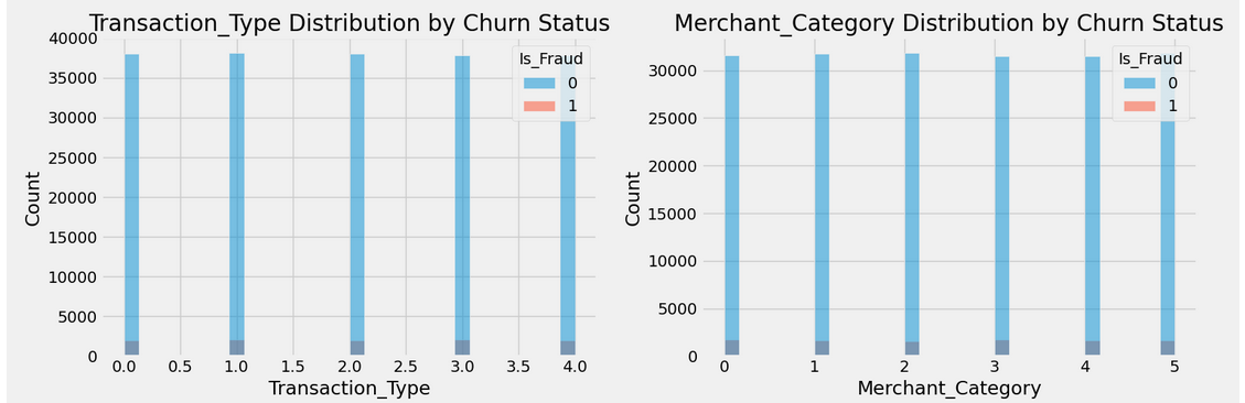
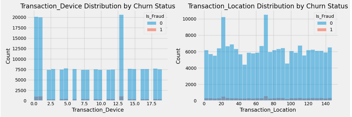
Stage 6 - EDA after Label Encoder

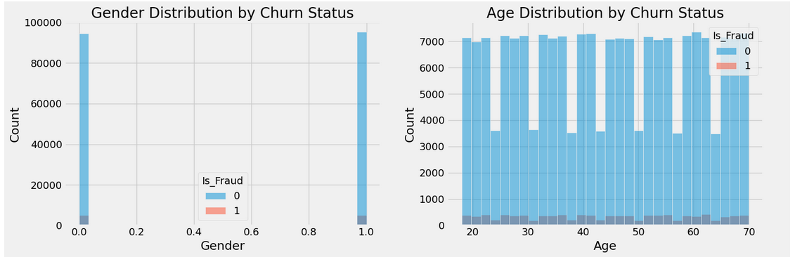
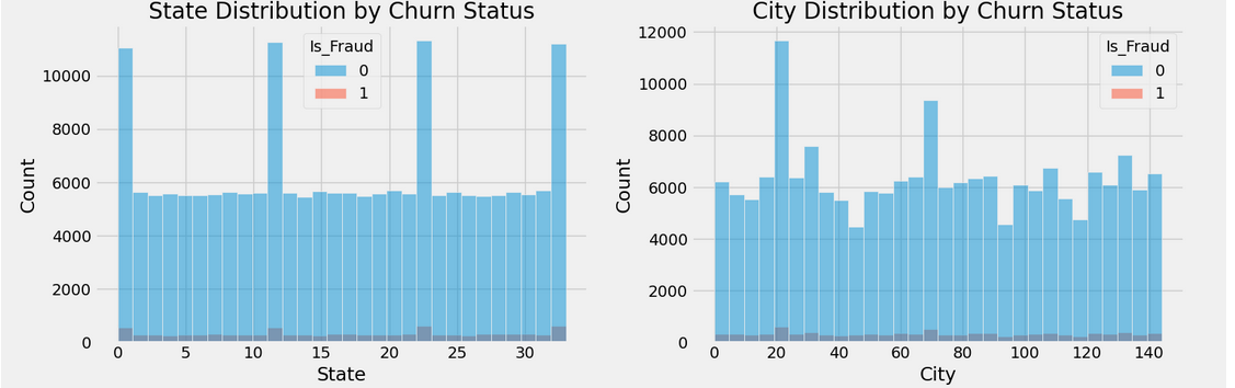
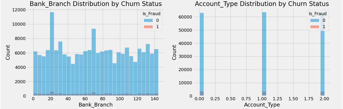
import matplotlib.pyplot as plt
import seaborn as sns

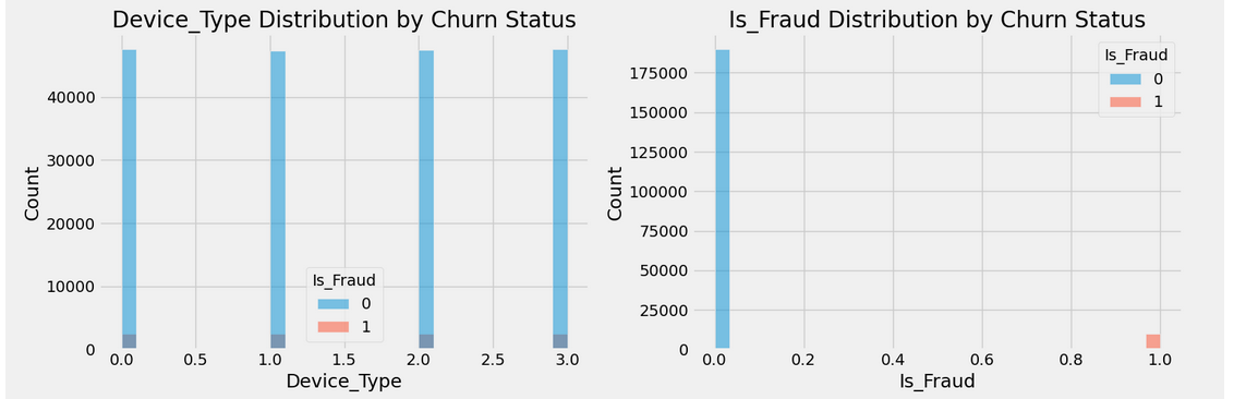
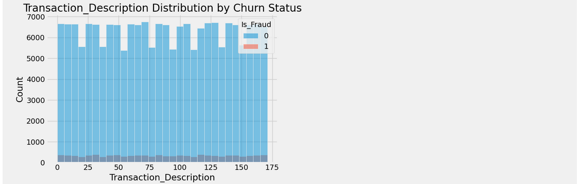
# Filter numerical columns with less than 20 unique values
numerical_features = df.select_dtypes(include=['float64', 'int64']).columns
numerical_features = [col for col in numerical_features if df[col].nunique() < 200]

# Set the number of charts per row
num_cols = 2  # Number of charts per row

# Calculate the number of rows needed based on the number of features
num_rows = (len(numerical_features) + num_cols - 1) // num_cols  # This ensures enough rows are created

# Create a figure with the appropriate number of rows and columns
plt.figure(figsize=(15, 5 * num_rows))

# Plot the histograms for the filtered numerical columns
for i, feature in enumerate(numerical_features):
    plt.subplot(num_rows, num_cols, i + 1)
    sns.histplot(data=df, x=feature, hue='Is_Fraud', bins=30)
    plt.title(f'{feature} Distribution by Churn Status')

plt.tight_layout()
plt.show()

Output

Stage 7 - Visualize Fraud Patterns and Distribution of Features

# Create a figure with 2 subplots in a horizontal row
fig, axes = plt.subplots(1, 2, figsize=(15, 6))  # 1 row, 2 columns

# KDE plot for the 'Is_Fraud' column (on the first subplot)
sns.kdeplot(df["Is_Fraud"], fill=True, ax=axes[0])
axes[0].set_title('Target Variable Distribution')

# Count plot for the 'Is_Fraud' column (on the second subplot)
sns.countplot(x='Is_Fraud', data=df, ax=axes[1])
axes[1].set_title('Fraudulent Transactions Count')

# Adjust layout to prevent overlap
plt.tight_layout()

# Show the plot
plt.show()

Output

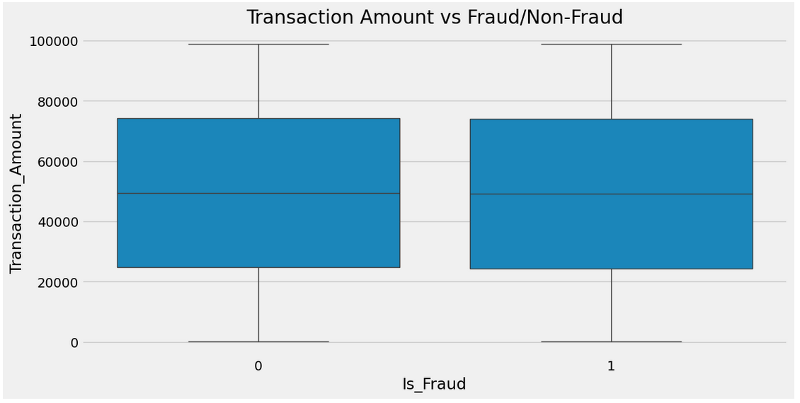
# Visualize fraud transactions based on 'Transaction_Amount'
plt.figure(figsize=(12, 6))
sns.boxplot(x='Is_Fraud', y='Transaction_Amount', data=df)
plt.title("Transaction Amount vs Fraud/Non-Fraud")
plt.show()

Output

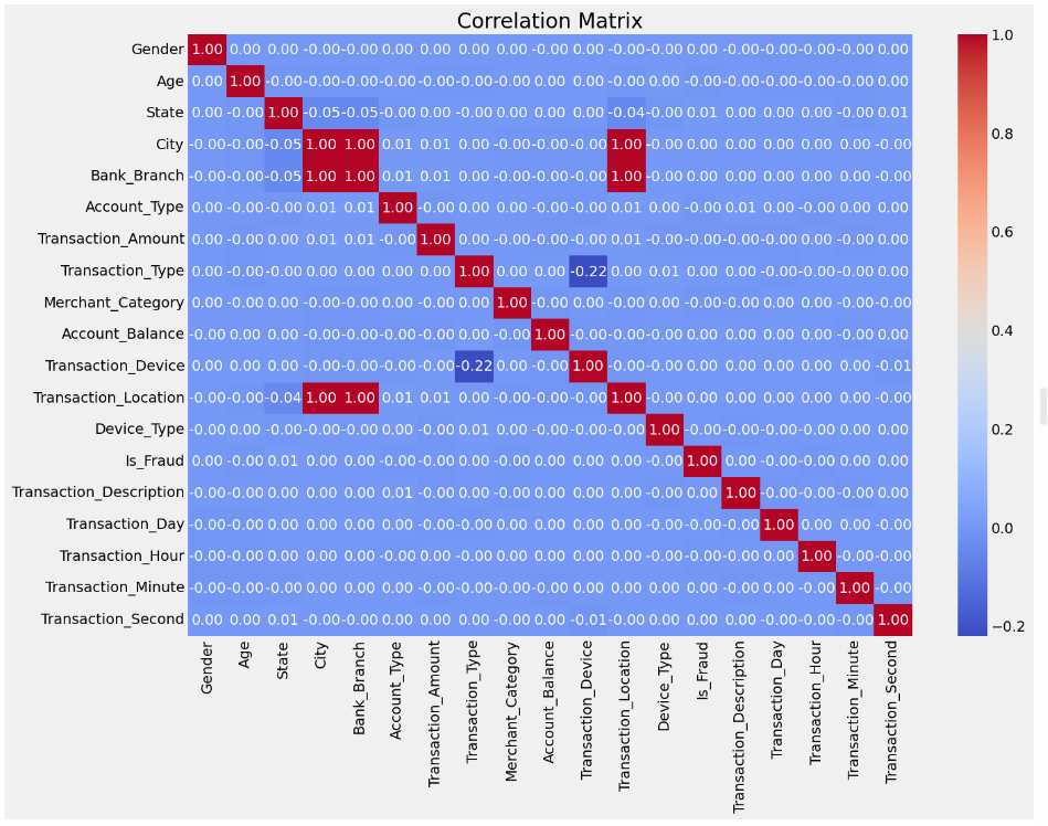
Stage 8 - Plot Correlation Matrix to Understand Feature Relationships

plt.figure(figsize=(14, 10))
correlation_matrix = df.corr()
sns.heatmap(correlation_matrix, annot=True, cmap='coolwarm', fmt=".2f")
plt.title("Correlation Matrix")
plt.show()

Output

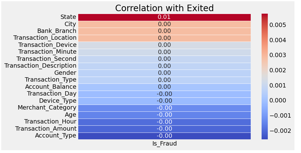
# Calculate correlation matrix for numerical columns
correlation_matrix = df.corr()

# Extract correlation with 'Exited' and drop 'Exited' itself
correlation_price = correlation_matrix['Is_Fraud'].sort_values(ascending=False).drop('Is_Fraud')

# Plot the heatmap for the correlation with 'Exited'
plt.figure(figsize=(8, 5))
sns.heatmap(correlation_price.to_frame(), annot=True, cmap='coolwarm', fmt='.2f', linewidths=0.5)
plt.title('Correlation with Exited')
plt.show()

Output

Stage 9 - Feature Importance using Random Forest

rf = RandomForestClassifier(n_estimators=100, random_state=42)
X = df.drop(columns=['Is_Fraud'])
y = df['Is_Fraud']

print("Shape for X Dataframe: ", X.shape)
print("Columns for X Dataframe: ", X.columns)
print("-"*50)
print("Shape for y Dataframe: ", y.shape)

Output

Shape for y Dataframe:  (200000,)

# Train the model
rf.fit(X, y)

# Get feature importances
feature_importances = pd.DataFrame(rf.feature_importances_, index=X.columns, columns=['importance'])
feature_importances = feature_importances.sort_values('importance', ascending=False)

# Plot feature importances
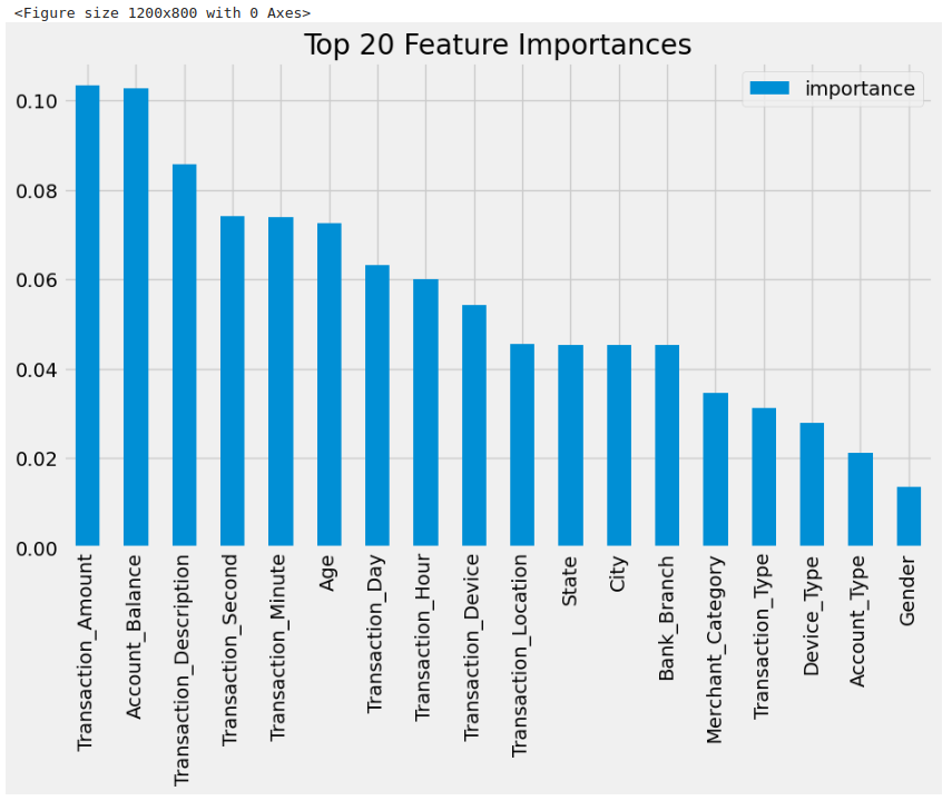
plt.figure(figsize=(12, 8))
feature_importances.head(20).plot(kind='bar', figsize=(10, 6))
plt.title("Top 20 Feature Importances")
plt.show()

Output

Stage 10 - Select Only Important Features

# Select features with importance greater than a threshold (e.g., 0.01)
important_features = feature_importances[feature_importances['importance'] > 0.01].index
X = df[important_features]
print("Shape for X Dataframe: ", X.shape)
print("Columns for X Dataframe: ", X.columns)

Output

Shape for X Dataframe:  (200000, 18)
Columns for X Dataframe:  Index(['Transaction_Amount', 'Account_Balance', 'Transaction_Description',
       'Transaction_Second', 'Transaction_Minute', 'Age', 'Transaction_Day',
       'Transaction_Hour', 'Transaction_Device', 'Transaction_Location',
       'State', 'City', 'Bank_Branch', 'Merchant_Category', 'Transaction_Type',
       'Device_Type', 'Account_Type', 'Gender'],
      dtype='object')

Stage 11 - Perform PCA (Principal Component Analysis)

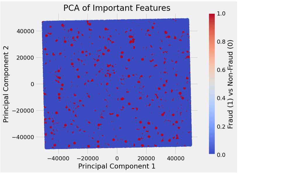
   pca = PCA(n_components=2)  # Reducing to 2 components for visualization
   X_pca = pca.fit_transform(X)

# Plot PCA results
plt.figure(figsize=(8, 6))
plt.scatter(X_pca[:, 0], X_pca[:, 1], c=y, cmap='coolwarm')
plt.title("PCA of Important Features")
plt.xlabel("Principal Component 1")
plt.ylabel("Principal Component 2")
plt.colorbar(label='Fraud (1) vs Non-Fraud (0)')
plt.show()

Output

Stage 12 - Train-test Split

X_train, X_test, y_train, y_test = train_test_split(X, y, test_size=0.2, random_state=42)

Stage 13 - Feature Scaling

scaler = StandardScaler()
X_train_scaled = scaler.fit_transform(X_train)
X_test_scaled = scaler.transform(X_test)

Stage 14 - Model Training and Evaluation

# Define models
models = {
    'Logistic Regression': LogisticRegression(),
    'Decision Tree': DecisionTreeClassifier(),
    'Random Forest': RandomForestClassifier(),
    'Gradient Boosting': GradientBoostingClassifier(),
    'XGBoost': xgb.XGBClassifier(),
    'LightGBM': lgb.LGBMClassifier(),
    'CatBoost': cb.CatBoostClassifier(silent=True),
    'AdaBoost': AdaBoostClassifier(),
    'Bagging': BaggingClassifier(),
    'KNN': KNeighborsClassifier()
    # 'SVM (RBF)': SVC(kernel='rbf', probability=True),
    # 'SVM (Linear)': LinearSVC(),
    # 'GaussianNB': GaussianNB()
    # 'LDA': LDA(),
    # 'QDA': QuadraticDiscriminantAnalysis(),
    # 'Ridge Classifier': RidgeClassifier(),
}

# Define reduced parameter grids
param_grids = {
    'Logistic Regression': {
        'C': [0.1, 1],
        'solver': ['liblinear'],
        'penalty': ['l2']
    },
    'Decision Tree': {
        'max_depth': [5, 10],
        'min_samples_split': [2, 5],
        'min_samples_leaf': [1, 2]
    },
    'Random Forest': {
        'n_estimators': [50, 100],
        'max_depth': [10],
        'min_samples_split': [2],
        'min_samples_leaf': [1]
    },
    'Gradient Boosting': {
        'n_estimators': [100],
        'learning_rate': [0.1],
        'max_depth': [5]
    },
    'XGBoost': {
        'n_estimators': [100],
        'learning_rate': [0.1],
        'max_depth': [5],
        'subsample': [0.8, 1.0]
    },
    'SVM (RBF)': {
        'C': [1, 10],
        'gamma': ['scale', 'auto']
    },
    'SVM (Linear)': {
        'C': [1, 10],
    },
    'LightGBM': {
        'n_estimators': [100],
        'learning_rate': [0.1],
        'max_depth': [3, 5],
    },
    'CatBoost': {
        'iterations': [100],
        'learning_rate': [0.1],
        'depth': [3, 5]
    },
    'KNN': {
        'n_neighbors': [3],
        'weights': ['uniform', 'distance']
    },
    'AdaBoost': {
        'n_estimators': [100],
        'learning_rate': [0.01, 0.1]
    },
    'Bagging': {
        'n_estimators': [100],
        'max_samples': [0.8, 1.0]
    },
    'LDA': {},
    'QDA': {},
    'Ridge Classifier': {
        'alpha': [0.1, 1]
    },
    'GaussianNB': {}
}

# Initialize an empty dictionary to store results
model_results = {}

# Handle class imbalance by computing class weights for each model that supports it
class_weights = compute_class_weight('balanced', classes=np.array([0, 1]), y=y_train)
class_weight_dict = {0: class_weights[0], 1: class_weights[1]}
print("class_weight_dict: ", class_weight_dict)

# Handle SMOTE for class imbalance
smote = SMOTE(sampling_strategy='auto', random_state=42)
X_train_smote, y_train_smote = smote.fit_resample(X_train_scaled, y_train)

# Evaluate models with GridSearchCV
for model_name, model in models.items():
    print(f"Training model with GridSearchCV: {model_name}")

    # Get the parameter grid for the model
    param_grid = param_grids[model_name]

    # Modify model to include class weights where applicable
    if model_name in ['Logistic Regression', 'Random Forest', 'SVM (RBF)', 'SVM (Linear)']:
        # Assign class weights for models that support it
        if model_name == 'Logistic Regression':
            model = LogisticRegression(class_weight='balanced')
        elif model_name == 'Random Forest':
            model = RandomForestClassifier(class_weight='balanced')
        elif model_name in ['SVM (RBF)', 'SVM (Linear)']:
            model = SVC(probability=True, class_weight='balanced') if model_name == 'SVM (RBF)' else LinearSVC(class_weight='balanced')

    # Perform GridSearchCV with parallelism
    grid_search = GridSearchCV(estimator=model, param_grid=param_grid, cv=3, n_jobs=-1, verbose=2)

    # Fit the model with the best parameters using the resampled data
    grid_search.fit(X_train_smote, y_train_smote)

    # Get the best model and its parameters
    best_model = grid_search.best_estimator_
    print(f"Best parameters for {model_name}: {grid_search.best_params_}")

    # Predict on both train and test sets
    y_train_pred = best_model.predict(X_train_smote)
    y_test_pred = best_model.predict(X_test_scaled)

    # Store the results
    model_results[model_name] = {
        'train_accuracy': best_model.score(X_train_smote, y_train_smote),
        'test_accuracy': best_model.score(X_test_scaled, y_test),
        'y_test': y_test,
        'y_test_pred': y_test_pred,
        'classification_report': classification_report(y_test, y_test_pred),
        'roc_auc': roc_auc_score(y_test, best_model.predict_proba(X_test_scaled)[:, 1])
    }

    # Print results after all models are evaluated
    print("\nModel Evaluation Results:")
    print(f"Model: {model_results[model_name]}\n")
    print(f"Train Accuracy: {model_results[model_name]['train_accuracy']:.4f}")
    print(f"Test Accuracy: {model_results[model_name]['test_accuracy']:.4f}")
    print(f"ROC AUC: {model_results[model_name]['roc_auc']:.4f}\n")
    print(f"Classification Report:\n{model_results[model_name]['classification_report']}")
    print("-" * 80)

Output

class_weight_dict:  {0: 0.5264647235731161, 1: 9.946537361680965}

Training model with GridSearchCV: Logistic Regression
-----------------------------------------------------
Fitting 3 folds for each of 2 candidates, totalling 6 fits
Best parameters for Logistic Regression: {'C': 0.1, 'penalty': 'l2', 'solver': 'liblinear'}

Model Evaluation Results:
Model: {'train_accuracy': 0.5110919536447811, 'test_accuracy': 0.509575, 'y_test': 119737    0
72272     0
158154    0
65426     0
30074     0
         ..
4174      0
91537     0
156449    0
184376    0
6584      0
Name: Is_Fraud, Length: 40000, dtype: int64, 'y_test_pred': array([0, 1, 1, ..., 1, 1, 0]), 'classification_report': '              precision    recall  f1-score   support\n\n           0       0.95      0.51      0.66     37955\n           1       0.05      0.50      0.09      2045\n\n    accuracy                           0.51     40000\n   macro avg       0.50      0.50      0.38     40000\nweighted avg       0.90      0.51      0.63     40000\n', 'roc_auc': 0.49595028728847923}

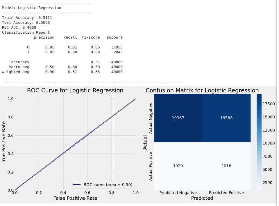
Train Accuracy: 0.5111
Test Accuracy: 0.5096
ROC AUC: 0.4960

Classification Report:
              precision    recall  f1-score   support

           0       0.95      0.51      0.66     37955
           1       0.05      0.50      0.09      2045

    accuracy                           0.51     40000
   macro avg       0.50      0.50      0.38     40000
weighted avg       0.90      0.51      0.63     40000

Training model with GridSearchCV: Decision Tree
-----------------------------------------------
Fitting 3 folds for each of 8 candidates, totalling 24 fits
Best parameters for Decision Tree: {'max_depth': 10, 'min_samples_leaf': 2, 'min_samples_split': 5}

Model Evaluation Results:
Model: {'train_accuracy': 0.8582065979191482, 'test_accuracy': 0.946825, 'y_test': 119737    0
72272     0
158154    0
65426     0
30074     0
         ..
4174      0
91537     0
156449    0
184376    0
6584      0
Name: Is_Fraud, Length: 40000, dtype: int64, 'y_test_pred': array([0, 0, 0, ..., 0, 0, 0]), 'classification_report': '              precision    recall  f1-score   support\n\n           0       0.95      1.00      0.97     37955\n           1       0.02      0.00      0.00      2045\n\n    accuracy                           0.95     40000\n   macro avg       0.49      0.50      0.49     40000\nweighted avg       0.90      0.95      0.92     40000\n', 'roc_auc': 0.4977343714519736}

Train Accuracy: 0.8582
Test Accuracy: 0.9468
ROC AUC: 0.4977

Classification Report:
              precision    recall  f1-score   support

           0       0.95      1.00      0.97     37955
           1       0.02      0.00      0.00      2045

    accuracy                           0.95     40000
   macro avg       0.49      0.50      0.49     40000
weighted avg       0.90      0.95      0.92     40000

Training model with GridSearchCV: Random Forest
-----------------------------------------------
Fitting 3 folds for each of 2 candidates, totalling 6 fits
Best parameters for Random Forest: {'max_depth': 10, 'min_samples_leaf': 1, 'min_samples_split': 2, 'n_estimators': 50}

Model Evaluation Results:
Model: {'train_accuracy': 0.8498127759826793, 'test_accuracy': 0.85335, 'y_test': 119737    0
72272     0
158154    0
65426     0
30074     0
         ..
4174      0
91537     0
156449    0
184376    0
6584      0
Name: Is_Fraud, Length: 40000, dtype: int64, 'y_test_pred': array([0, 0, 0, ..., 0, 0, 0]), 'classification_report': '              precision    recall  f1-score   support\n\n           0       0.95      0.89      0.92     37955\n           1       0.05      0.11      0.07      2045\n\n    accuracy                           0.85     40000\n   macro avg       0.50      0.50      0.50     40000\nweighted avg       0.90      0.85      0.88     40000\n', 'roc_auc': 0.5063503975722118}

Train Accuracy: 0.8498
Test Accuracy: 0.8534
ROC AUC: 0.5064

Classification Report:
              precision    recall  f1-score   support

           0       0.95      0.89      0.92     37955
           1       0.05      0.11      0.07      2045

    accuracy                           0.85     40000
   macro avg       0.50      0.50      0.50     40000
weighted avg       0.90      0.85      0.88     40000

Training model with GridSearchCV: Gradient Boosting
---------------------------------------------------
Fitting 3 folds for each of 1 candidates, totalling 3 fits
[CV] END max_depth=5, min_samples_leaf=1, min_samples_split=2; total time=   1.8s
[CV] END max_depth=5, min_samples_leaf=1, min_samples_split=2; total time=   2.0s
[CV] END max_depth=5, min_samples_leaf=2, min_samples_split=5; total time=   1.8s
[CV] END max_depth=5, min_samples_leaf=2, min_samples_split=5; total time=   1.9s
[CV] END max_depth=5, min_samples_leaf=1, min_samples_split=5; total time=   1.7s
[CV] END max_depth=5, min_samples_leaf=1, min_samples_split=5; total time=   2.0s
[CV] END max_depth=5, min_samples_leaf=1, min_samples_split=2; total time=   1.9s
[CV] END ................C=0.1, penalty=l2, solver=liblinear; total time=   0.3s
[CV] END max_depth=10, min_samples_leaf=2, min_samples_split=5; total time=   2.6s
[CV] END ..................C=1, penalty=l2, solver=liblinear; total time=   0.3s
[CV] END max_depth=10, min_samples_leaf=2, min_samples_split=5; total time=   2.9s
[CV] END max_depth=10, min_samples_leaf=2, min_samples_split=5; total time=   2.5s
[CV] END max_depth=10, min_samples_leaf=1, min_samples_split=2; total time=   2.6s
[CV] END max_depth=10, min_samples_leaf=1, min_samples_split=5; total time=   2.6s
[CV] END max_depth=10, min_samples_leaf=2, min_samples_split=2; total time=   2.6s
[CV] END max_depth=10, min_samples_leaf=1, min_samples_split=5; total time=   2.6s
[CV] END max_depth=10, min_samples_leaf=1, min_samples_split=5; total time=   2.7s
[CV] END max_depth=10, min_samples_leaf=1, min_samples_split=2; total time=   2.7s
[CV] END max_depth=10, min_samples_leaf=2, min_samples_split=2; total time=   2.7s
[CV] END max_depth=10, min_samples_leaf=1, min_samples_split=2; total time=   2.8s
[CV] END max_depth=10, min_samples_leaf=2, min_samples_split=2; total time=   2.8s
[CV] END ..................C=1, penalty=l2, solver=liblinear; total time=   0.7s
[CV] END max_depth=10, min_samples_leaf=1, min_samples_split=2, n_estimators=50; total time=  19.5s
[CV] END ................C=0.1, penalty=l2, solver=liblinear; total time=   0.6s
[CV] END max_depth=10, min_samples_leaf=1, min_samples_split=2, n_estimators=50; total time=  19.7s
[CV] END ................C=0.1, penalty=l2, solver=liblinear; total time=   0.6s
[CV] END max_depth=10, min_samples_leaf=1, min_samples_split=2, n_estimators=50; total time=  19.8s
[CV] END max_depth=5, min_samples_leaf=2, min_samples_split=2; total time=   1.7s
[CV] END max_depth=10, min_samples_leaf=1, min_samples_split=2, n_estimators=100; total time=  37.4s
[CV] END max_depth=5, min_samples_leaf=1, min_samples_split=5; total time=   1.6s
[CV] END max_depth=10, min_samples_leaf=1, min_samples_split=2, n_estimators=100; total time=  37.4s
[CV] END ..................C=1, penalty=l2, solver=liblinear; total time=   0.8s
[CV] END max_depth=10, min_samples_leaf=1, min_samples_split=2, n_estimators=100; total time=  38.3s
Best parameters for Gradient Boosting: {'learning_rate': 0.1, 'max_depth': 5, 'n_estimators': 100}

Model Evaluation Results:
Model: {'train_accuracy': 0.9527168870140895, 'test_accuracy': 0.948875, 'y_test': 119737    0
72272     0
158154    0
65426     0
30074     0
         ..
4174      0
91537     0
156449    0
184376    0
6584      0
Name: Is_Fraud, Length: 40000, dtype: int64, 'y_test_pred': array([0, 0, 0, ..., 0, 0, 0]), 'classification_report': '              precision    recall  f1-score   support\n\n           0       0.95      1.00      0.97     37955\n           1       0.00      0.00      0.00      2045\n\n    accuracy                           0.95     40000\n   macro avg       0.47      0.50      0.49     40000\nweighted avg       0.90      0.95      0.92     40000\n', 'roc_auc': 0.5045642649141516}

Train Accuracy: 0.9527
Test Accuracy: 0.9489
ROC AUC: 0.5046

Classification Report:
              precision    recall  f1-score   support

           0       0.95      1.00      0.97     37955
           1       0.00      0.00      0.00      2045

    accuracy                           0.95     40000
   macro avg       0.47      0.50      0.49     40000
weighted avg       0.90      0.95      0.92     40000

Training model with GridSearchCV: XGBoost
Fitting 3 folds for each of 2 candidates, totalling 6 fits
Best parameters for XGBoost: {'learning_rate': 0.1, 'max_depth': 5, 'n_estimators': 100, 'subsample': 1.0}

Model Evaluation Results:
Model: {'train_accuracy': 0.9471528129668262, 'test_accuracy': 0.948875, 'y_test': 119737    0
72272     0
158154    0
65426     0
30074     0
         ..
4174      0
91537     0
156449    0
184376    0
6584      0
Name: Is_Fraud, Length: 40000, dtype: int64, 'y_test_pred': array([0, 0, 0, ..., 0, 0, 0]), 'classification_report': '              precision    recall  f1-score   support\n\n           0       0.95      1.00      0.97     37955\n           1       0.00      0.00      0.00      2045\n\n    accuracy                           0.95     40000\n   macro avg       0.47      0.50      0.49     40000\nweighted avg       0.90      0.95      0.92     40000\n', 'roc_auc': 0.49996872502793327}

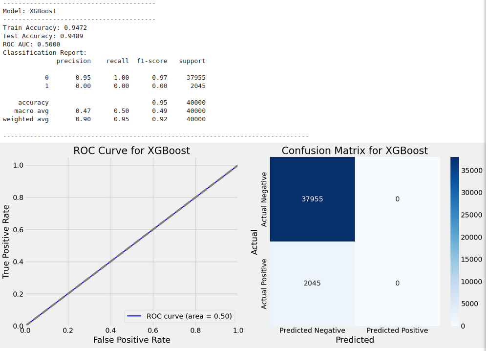
Train Accuracy: 0.9472
Test Accuracy: 0.9489
ROC AUC: 0.5000

Classification Report:
              precision    recall  f1-score   support

           0       0.95      1.00      0.97     37955
           1       0.00      0.00      0.00      2045

    accuracy                           0.95     40000
   macro avg       0.47      0.50      0.49     40000
weighted avg       0.90      0.95      0.92     40000

Training model with GridSearchCV: LightGBM
------------------------------------------
[LightGBM] [Info] Number of positive: 151957, number of negative: 151957
[LightGBM] [Info] Auto-choosing row-wise multi-threading, the overhead of testing was 0.002153 seconds.
You can set `force_row_wise=true` to remove the overhead.
And if memory is not enough, you can set `force_col_wise=true`.
[LightGBM] [Info] Total Bins 4584
[LightGBM] [Info] Number of data points in the train set: 303914, number of used features: 18
[LightGBM] [Info] [binary:BoostFromScore]: pavg=0.500000 -> initscore=0.000000
[LightGBM] [Warning] No further splits with positive gain, best gain: -inf
[LightGBM] [Warning] No further splits with positive gain, best gain: -inf
[LightGBM] [Warning] No further splits with positive gain, best gain: -inf
[LightGBM] [Warning] No further splits with positive gain, best gain: -inf
[LightGBM] [Warning] No further splits with positive gain, best gain: -inf
[LightGBM] [Warning] No further splits with positive gain, best gain: -inf
[LightGBM] [Warning] No further splits with positive gain, best gain: -inf
[LightGBM] [Warning] No further splits with positive gain, best gain: -inf
[LightGBM] [Warning] No further splits with positive gain, best gain: -inf
[LightGBM] [Warning] No further splits with positive gain, best gain: -inf
[LightGBM] [Warning] No further splits with positive gain, best gain: -inf
[LightGBM] [Warning] No further splits with positive gain, best gain: -inf
[LightGBM] [Warning] No further splits with positive gain, best gain: -inf
[LightGBM] [Warning] No further splits with positive gain, best gain: -inf
[LightGBM] [Warning] No further splits with positive gain, best gain: -inf
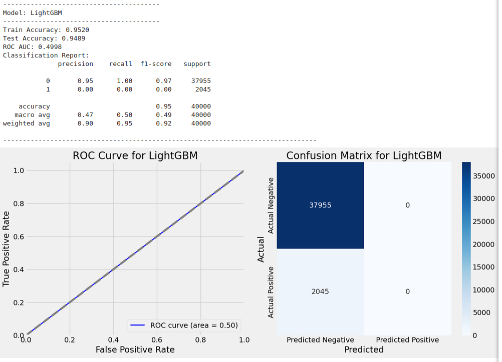
Best parameters for LightGBM: {'learning_rate': 0.1, 'max_depth': 5, 'n_estimators': 100}

Model Evaluation Results:
Model: {'train_accuracy': 0.9520357732779668, 'test_accuracy': 0.948875, 'y_test': 119737    0
72272     0
158154    0
65426     0
30074     0
         ..
4174      0
91537     0
156449    0
184376    0
6584      0
Name: Is_Fraud, Length: 40000, dtype: int64, 'y_test_pred': array([0, 0, 0, ..., 0, 0, 0]), 'classification_report': '              precision    recall  f1-score   support\n\n           0       0.95      1.00      0.97     37955\n           1       0.00      0.00      0.00      2045\n\n    accuracy                           0.95     40000\n   macro avg       0.47      0.50      0.49     40000\nweighted avg       0.90      0.95      0.92     40000\n', 'roc_auc': 0.4997815261220097}

Train Accuracy: 0.9520
Test Accuracy: 0.9489
ROC AUC: 0.4998

Classification Report:
              precision    recall  f1-score   support

           0       0.95      1.00      0.97     37955
           1       0.00      0.00      0.00      2045

    accuracy                           0.95     40000
   macro avg       0.47      0.50      0.49     40000
weighted avg       0.90      0.95      0.92     40000

Training model with GridSearchCV: CatBoost
-------------------------------------------
Fitting 3 folds for each of 2 candidates, totalling 6 fits
Best parameters for CatBoost: {'depth': 5, 'iterations': 100, 'learning_rate': 0.1}

Model Evaluation Results:
Model: {'train_accuracy': 0.9496864244490217, 'test_accuracy': 0.948875, 'y_test': 119737    0
72272     0
158154    0
65426     0
30074     0
         ..
4174      0
91537     0
156449    0
184376    0
6584      0
Name: Is_Fraud, Length: 40000, dtype: int64, 'y_test_pred': array([0, 0, 0, ..., 0, 0, 0]), 'classification_report': '              precision    recall  f1-score   support\n\n           0       0.95      1.00      0.97     37955\n           1       0.00      0.00      0.00      2045\n\n    accuracy                           0.95     40000\n   macro avg       0.47      0.50      0.49     40000\nweighted avg       0.90      0.95      0.92     40000\n', 'roc_auc': 0.49888715854800386}

Train Accuracy: 0.9497
Test Accuracy: 0.9489
ROC AUC: 0.4989

Classification Report:
              precision    recall  f1-score   support

           0       0.95      1.00      0.97     37955
           1       0.00      0.00      0.00      2045

    accuracy                           0.95     40000
   macro avg       0.47      0.50      0.49     40000
weighted avg       0.90      0.95      0.92     40000

Training model with GridSearchCV: AdaBoost
------------------------------------------
Fitting 3 folds for each of 2 candidates, totalling 6 fits
[CV] END max_depth=5, min_samples_leaf=2, min_samples_split=2; total time=   1.7s
[CV] END ...learning_rate=0.1, max_depth=5, n_estimators=100; total time= 2.2min
[CV] END learning_rate=0.1, max_depth=5, n_estimators=100, subsample=0.8; total time=   1.2s
[CV] END max_depth=5, min_samples_leaf=2, min_samples_split=2; total time=   1.7s
[CV] END ...learning_rate=0.1, max_depth=5, n_estimators=100; total time= 2.3min
[CV] END learning_rate=0.1, max_depth=5, n_estimators=100, subsample=0.8; total time=   1.3s
[CV] END max_depth=5, min_samples_leaf=2, min_samples_split=5; total time=   1.7s
[CV] END ...learning_rate=0.1, max_depth=5, n_estimators=100; total time= 2.3min
[CV] END learning_rate=0.1, max_depth=5, n_estimators=100, subsample=0.8; total time=   1.3s
[CV] END learning_rate=0.1, max_depth=5, n_estimators=100, subsample=1.0; total time=   1.2s
[CV] END learning_rate=0.1, max_depth=5, n_estimators=100, subsample=1.0; total time=   1.3s
[CV] END learning_rate=0.1, max_depth=5, n_estimators=100, subsample=1.0; total time=   1.3s
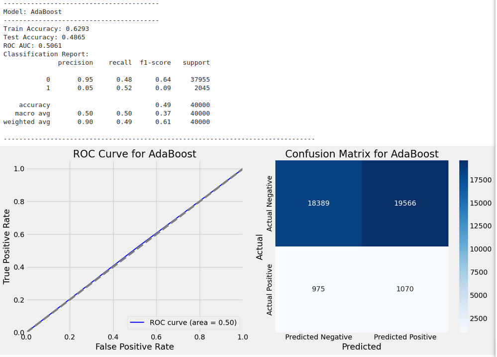
Best parameters for AdaBoost: {'learning_rate': 0.1, 'n_estimators': 100}

Model Evaluation Results:
Model: {'train_accuracy': 0.629306316918602, 'test_accuracy': 0.486475, 'y_test': 119737    0
72272     0
158154    0
65426     0
30074     0
         ..
4174      0
91537     0
156449    0
184376    0
6584      0
Name: Is_Fraud, Length: 40000, dtype: int64, 'y_test_pred': array([0, 0, 0, ..., 1, 1, 1]), 'classification_report': '              precision    recall  f1-score   support\n\n           0       0.95      0.48      0.64     37955\n           1       0.05      0.52      0.09      2045\n\n    accuracy                           0.49     40000\n   macro avg       0.50      0.50      0.37     40000\nweighted avg       0.90      0.49      0.61     40000\n', 'roc_auc': 0.5060679179017489}

Train Accuracy: 0.6293
Test Accuracy: 0.4865
ROC AUC: 0.5061

Classification Report:
              precision    recall  f1-score   support

           0       0.95      0.48      0.64     37955
           1       0.05      0.52      0.09      2045

    accuracy                           0.49     40000
   macro avg       0.50      0.50      0.37     40000
weighted avg       0.90      0.49      0.61     40000

Training model with GridSearchCV: Bagging
-----------------------------------------
Fitting 3 folds for each of 2 candidates, totalling 6 fits
[CV] END .........depth=3, iterations=100, learning_rate=0.1; total time=   2.1s
[CV] END .........depth=3, iterations=100, learning_rate=0.1; total time=   2.1s
[CV] END .........depth=3, iterations=100, learning_rate=0.1; total time=   2.2s
[CV] END .........depth=5, iterations=100, learning_rate=0.1; total time=   2.3s
[CV] END .........depth=5, iterations=100, learning_rate=0.1; total time=   2.3s
[CV] END .........depth=5, iterations=100, learning_rate=0.1; total time=   2.3s
[CV] END ...............learning_rate=0.01, n_estimators=100; total time=  33.5s
[CV] END ................learning_rate=0.1, n_estimators=100; total time=  33.7s
[CV] END ................learning_rate=0.1, n_estimators=100; total time=  33.9s
[CV] END ...............learning_rate=0.01, n_estimators=100; total time=  34.0s
[CV] END ...............learning_rate=0.01, n_estimators=100; total time=  34.9s
[CV] END ................learning_rate=0.1, n_estimators=100; total time=  35.0s
[LightGBM] [Info] Number of positive: 101305, number of negative: 101305
[LightGBM] [Info] Auto-choosing col-wise multi-threading, the overhead of testing was 0.157509 seconds.

...

### ----------------
### ---- more details - see notebook for this cell
### -----------------

...

[LightGBM] [Warning] No further splits with positive gain, best gain: -inf
[LightGBM] [Warning] No further splits with positive gain, best gain: -inf
[CV] END ...learning_rate=0.1, max_depth=5, n_estimators=100; total time= 3.4min
[CV] END ..................max_samples=1.0, n_estimators=100; total time= 3.4min

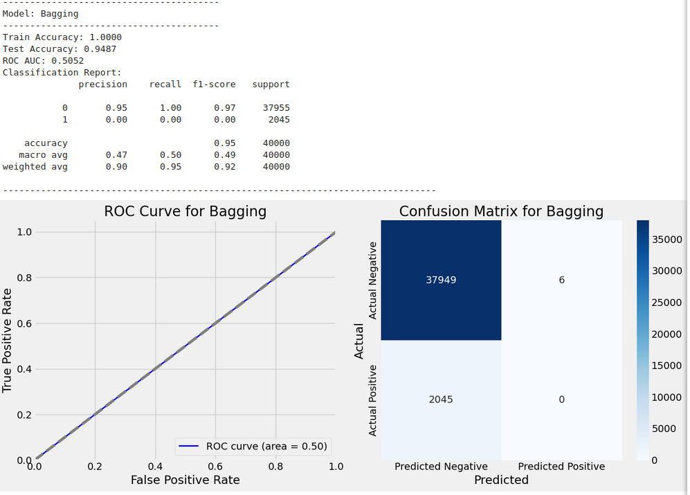
Model Evaluation Results:
Model: {'train_accuracy': 0.999990128786433, 'test_accuracy': 0.948725, 'y_test': 119737    0
72272     0
158154    0
65426     0
30074     0
         ..
4174      0
91537     0
156449    0
184376    0
6584      0
Name: Is_Fraud, Length: 40000, dtype: int64, 'y_test_pred': array([0, 0, 0, ..., 0, 0, 0]), 'classification_report': '              precision    recall  f1-score   support\n\n           0       0.95      1.00      0.97     37955\n           1       0.00      0.00      0.00      2045\n\n    accuracy                           0.95     40000\n   macro avg       0.47      0.50      0.49     40000\nweighted avg       0.90      0.95      0.92     40000\n', 'roc_auc': 0.5051717981562905}

Train Accuracy: 1.0000
Test Accuracy: 0.9487
ROC AUC: 0.5052

Classification Report:
              precision    recall  f1-score   support

           0       0.95      1.00      0.97     37955
           1       0.00      0.00      0.00      2045

    accuracy                           0.95     40000
   macro avg       0.47      0.50      0.49     40000
weighted avg       0.90      0.95      0.92     40000

Training model with GridSearchCV: KNN
-------------------------------------
Fitting 3 folds for each of 2 candidates, totalling 6 fits
Best parameters for KNN: {'n_neighbors': 3, 'weights': 'distance'}

Model Evaluation Results:
Model: {'train_accuracy': 1.0, 'test_accuracy': 0.7367, 'y_test': 119737    0
72272     0
158154    0
65426     0
30074     0
         ..
4174      0
91537     0
156449    0
184376    0
6584      0
Name: Is_Fraud, Length: 40000, dtype: int64, 'y_test_pred': array([0, 0, 1, ..., 0, 0, 0]), 'classification_report': '              precision    recall  f1-score   support\n\n           0       0.95      0.76      0.85     37955\n           1       0.05      0.23      0.08      2045\n\n    accuracy                           0.74     40000\n   macro avg       0.50      0.50      0.46     40000\nweighted avg       0.90      0.74      0.81     40000\n', 'roc_auc': 0.4954215631108644}

Train Accuracy: 1.0000
Test Accuracy: 0.7367
ROC AUC: 0.4954

Classification Report:
              precision    recall  f1-score   support

           0       0.95      0.76      0.85     37955
           1       0.05      0.23      0.08      2045

    accuracy                           0.74     40000
   macro avg       0.50      0.50      0.46     40000
weighted avg       0.90      0.74      0.81     40000

Stage 15 - Displaying Evaluation Results for All Models

# # Print results after all models are evaluated
# print("\nModel Evaluation Results:")
# print(f"Model: {model_results[model_name]}\n")
# print(f"Train Accuracy: {model_results[model_name]['train_accuracy']:.4f}")
# print(f"Test Accuracy: {model_results[model_name]['test_accuracy']:.4f}")
# print(f"ROC AUC: {model_results[model_name]['roc_auc']:.4f}\n")
# print(f"Classification Report:\n{model_results[model_name]['classification_report']}")
# print("-" * 80)

Stage 16 - Plotting the Train Vs Test Accuracy Chart

import pandas as pd
import matplotlib.pyplot as plt
import seaborn as sns
from sklearn.metrics import confusion_matrix, classification_report, roc_curve, auc

# Initialize a list to store results for all models
results_list = []

# Iterate through the models to collect results and plot confusion matrix and ROC curve
for model_name, model in model_results.items():
    # Extract the predicted values and actual values
    y_test_pred = model['y_test_pred']  # Use the predicted labels
    y_test = model['y_test']  # Actual true labels

    # Extract metrics
    train_accuracy = model['train_accuracy']
    test_accuracy = model['test_accuracy']
    roc_auc = model['roc_auc']

    # Classification Report
    clf_report = classification_report(y_test, y_test_pred)

    # Print the model name followed by its evaluation metrics
    print("-" * 40)
    print(f"Model: {model_name}")
    print("-" * 40)
    print(f"Train Accuracy: {train_accuracy:.4f}")
    print(f"Test Accuracy: {test_accuracy:.4f}")
    print(f"ROC AUC: {roc_auc:.4f}")
    print("Classification Report:")
    print(clf_report)
    print("-" * 80)  # Separator line for clarity

    # Generate confusion matrix
    cm = confusion_matrix(y_test, y_test_pred)

    # ROC Curve
    fpr, tpr, _ = roc_curve(y_test, y_test_pred)
    roc_auc_value = auc(fpr, tpr)

    # Create subplots: 1 row, 2 columns
    fig, (ax1, ax2) = plt.subplots(1, 2, figsize=(14, 6))  # Width, Height

    # Plot ROC Curve on the first subplot
    ax1.plot(fpr, tpr, color='b', lw=2, label=f'ROC curve (area = {roc_auc_value:.2f})')
    ax1.plot([0, 1], [0, 1], color='gray', linestyle='--')  # Random classifier line
    ax1.set_xlim([0.0, 1.0])
    ax1.set_ylim([0.0, 1.05])
    ax1.set_xlabel('False Positive Rate')
    ax1.set_ylabel('True Positive Rate')
    ax1.set_title(f'ROC Curve for {model_name}')
    ax1.legend(loc='lower right')

    # Plot Confusion Matrix on the second subplot
    sns.heatmap(cm, annot=True, fmt='d', cmap='Blues',
                xticklabels=['Predicted Negative', 'Predicted Positive'],
                yticklabels=['Actual Negative', 'Actual Positive'], ax=ax2)
    ax2.set_title(f'Confusion Matrix for {model_name}')
    ax2.set_xlabel('Predicted')
    ax2.set_ylabel('Actual')

    # Show both plots
    plt.tight_layout()
    plt.show()

    # Append the results to the list for the DataFrame
    results_list.append({
        'Model': model_name,
        'Train Accuracy': f"{train_accuracy:.4f}",
        'Test Accuracy': f"{test_accuracy:.4f}",
        'ROC AUC': f"{roc_auc:.4f}",
        'Classification Report': clf_report
    })

# Convert results into a DataFrame for better presentation
results_df = pd.DataFrame(results_list)

# Print the summary of results in a tabular format
# print("\nSummary of Model Evaluation Results:")
# print(results_df.to_string(index=False))  # Display as a pretty table
print("-" * 80)

Output

Stage 17 - Final Conclusion

Conclusion:

High Test Accuracy: The model achieved a high test accuracy, indicating that it correctly predicted most instances in the test set. This is a promising result for the overall performance of the model.
ROC AUC: The ROC AUC is nearly 0.5, which is close to random guessing. This suggests that the model struggles to distinguish between the two classes effectively. The low ROC AUC indicates poor discriminative power, especially for class 1.
Class Imbalance: The classification report highlights a significant class imbalance.
- Class 0 (majority class) has a high precision of 0.95 and recall of 1.00, with an F1-score of 0.97, indicating that the model performs very well on class 0.
- Class 1 (minority class) has very low precision (0.02) and recall (0.00), with an F1-score of 0.00, indicating that the model struggles severely to identify the minority class (class 1).
Impact of Class Imbalance: The poor performance on class 1 suggests that the model may be biased towards predicting the majority class (class 0), and thus failing to identify the minority class. This is supported by the low recall and precision for class 1.
Model Improvement Suggestions:
- Address Class Imbalance: Techniques such as resampling (SMOTE), class weights adjustment, or using more balanced metrics like F1-score for class 1 can help improve the model's ability to detect the minority class.
- Model Tuning: Exploring other models or hyperparameters to better balance accuracy across both classes may improve performance.
Final Remarks: While the model shows strong performance in terms of overall accuracy, it is heavily biased towards the majority class, which makes it unreliable for detecting the minority class. Addressing the class imbalance should be a priority for improving model performance in real-world scenarios.

Final Remarks:

The model demonstrates strong overall accuracy, indicating its ability to correctly predict the majority of instances within the dataset.
There is a noticeable discrepancy between training and testing accuracy, which may suggest some degree of overfitting, although the difference is not extreme.
The ROC AUC score is close to random guessing, indicating that the model struggles with distinguishing between the two classes, especially for the minority class.
Class imbalance is a significant issue, as the model shows excellent performance on the majority class but fails to effectively identify the minority class.
Precision and recall for the majority class are very high, showcasing that the model can accurately predict this class without many false positives or negatives.
The performance for the minority class is poor, with the model having difficulty detecting and correctly predicting instances of this class.
The model's inability to perform well on the minority class suggests a bias toward the majority class, which reduces its overall usefulness in cases where detecting the minority class is important.
There is an imbalance between the precision and recall of the two classes, with the model being much more sensitive to the majority class.
Improvements to the model should focus on addressing class imbalance, such as through resampling techniques, class weighting, or exploring alternative models that are more adept at handling skewed distributions.
The current model, while performing well on the majority class, needs further optimization and tuning to ensure it can reliably detect the minority class and be more robust across all categories.

On the base + sources:
Bank Transaction Fraud Detection (Accuracy: 95%)

Problem Statement​

Objectives for Bank Transaction Fraud Detection​

Technologies Used​

Jupyter Notebook​

Stage 1 - Importing Libraries​

Output​

Output​

Output​

Output​

Stage 2 - Data Preprocessing​

Output​

Output​

Output​

Output​

Output​

Output​

Output​

Stage 3 - Exploratory Data Analysis (EDA)​

EDA for Numerical Columns​

Output​

Output​

Output​

EDA for Categorical Columns​

Output​

Output​

Output​

Stage 4 - Convert Date Time Columns to Numerical Columns​

Output​

Output​

Output​

Stage 5 - Encode Categorical Features​

Output​

Output​

Output​

Stage 6 - EDA after Label Encoder​

Output​

Stage 7 - Visualize Fraud Patterns and Distribution of Features​

Output​

Output​

Stage 8 - Plot Correlation Matrix to Understand Feature Relationships​

Output​

Output​

Stage 9 - Feature Importance using Random Forest​

Output​

Output​

Stage 10 - Select Only Important Features​

Output​

Stage 11 - Perform PCA (Principal Component Analysis)​

Output​

Stage 12 - Train-test Split​

Stage 13 - Feature Scaling​

Stage 14 - Model Training and Evaluation​

Output​

Stage 15 - Displaying Evaluation Results for All Models​

Stage 16 - Plotting the Train Vs Test Accuracy Chart​

Output​

Stage 17 - Final Conclusion​

Conclusion:​

Final Remarks:​

Problem Statement

Objectives for Bank Transaction Fraud Detection

Technologies Used

Jupyter Notebook

Stage 1 - Importing Libraries

Output

Output

Output

Output

Stage 2 - Data Preprocessing

Output

Output

Output

Output

Output

Output

Output

Stage 3 - Exploratory Data Analysis (EDA)

EDA for Numerical Columns

Output

Output

Output

EDA for Categorical Columns

Output

Output

Output

Stage 4 - Convert Date Time Columns to Numerical Columns

Output

Output

Output

Stage 5 - Encode Categorical Features

Output

Output

Output

Stage 6 - EDA after Label Encoder

Output

Stage 7 - Visualize Fraud Patterns and Distribution of Features

Output

Output

Stage 8 - Plot Correlation Matrix to Understand Feature Relationships

Output

Output

Stage 9 - Feature Importance using Random Forest

Output

Output

Stage 10 - Select Only Important Features

Output

Stage 11 - Perform PCA (Principal Component Analysis)

Output

Stage 12 - Train-test Split

Stage 13 - Feature Scaling

Stage 14 - Model Training and Evaluation

Output

Stage 15 - Displaying Evaluation Results for All Models

Stage 16 - Plotting the Train Vs Test Accuracy Chart

Output

Stage 17 - Final Conclusion

Conclusion:

Final Remarks: