Tesla Stock Price Prediction
Objective and Overview
The primary objective of this analysis was to predict Tesla’s stock closing prices based on historical data. Using machine learning techniques, the goal was to evaluate the model's performance and make accurate predictions while identifying key drivers of stock price movements.
Steps Taken
Data Collection and Processing:
- Loaded historical Tesla stock price data.
- Preprocessed the data by cleaning columns (e.g., removing special characters like $) and converting them into numeric format.
- Checked for and handled missing values to ensure data integrity.
- Visualized Past Trend data before making my model to better grasp the volatility and trend visually
Model Training:
-
Created lagging features (Close_t-1, Close_t-2, etc.), moving averages (e.g., 7_day_avg, 30_day_avg), and volatility metrics (e.g., 7_day_volatility) to capture trends and patterns in stock prices.
- Split the dataset into training and testing sets using an 80-20 split.
- Trained a Random Forest Regressor as the predictive model.
- Evaluated the model on the test set using Mean Squared Error (MSE), achieving an MSE of 16.44, which translates to a Root Mean Squared Error (RMSE) of approximately $4.05.
Hyperparameter Tuning:
- Optimized the model by tuning key hyperparameters using RandomizedSearchCV to find the best configuration (e.g., number of trees, depth of trees, and minimum samples per split).
- Improved the model’s performance based on optimized parameters.
Feature Importance Analysis:
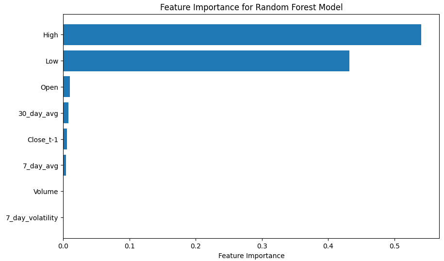
- Evaluated feature importance using the trained Random Forest model to understand which factors contributed most to predictions.
- Identified key features, such as previous day’s closing price (Close_t-1) and moving averages, as the most influential drivers of the model.
Model Visualization:
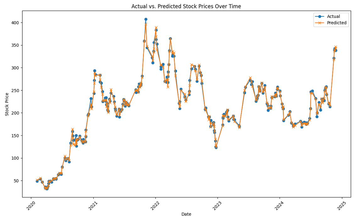
- Created visualizations to evaluate model performance: Actual vs. Predicted Stock Prices Over Time: Showed that the model accurately captures trends and movements in Tesla’s stock price.
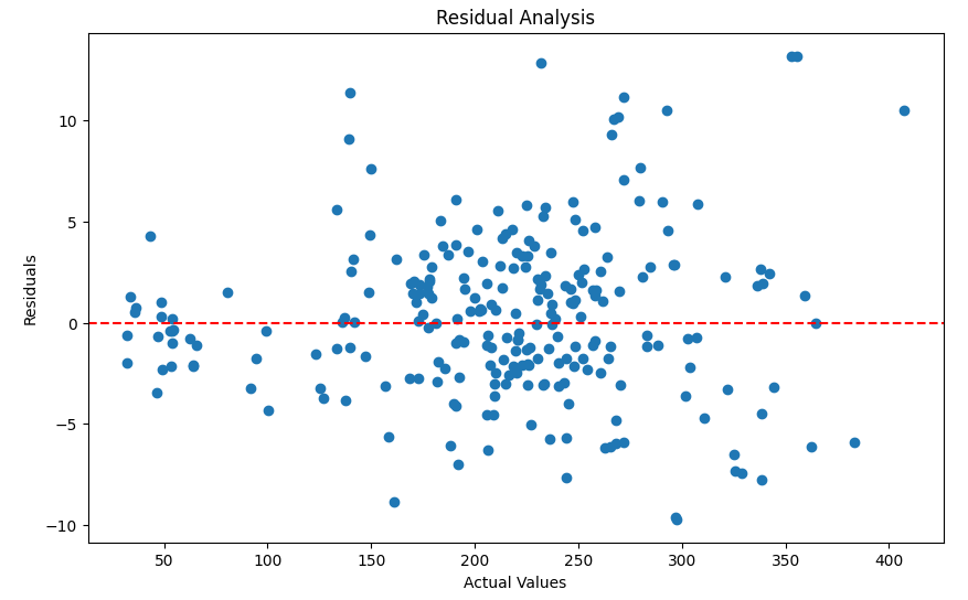
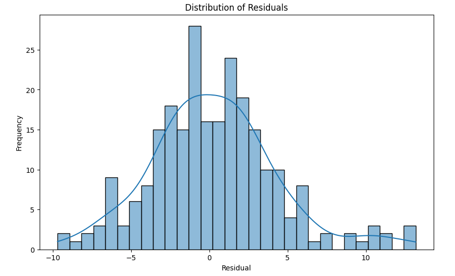
- Residual Plot: Confirmed that residuals were mostly randomly distributed around zero, indicating a lack of significant bias.
- Feature Importance Plot: Highlighted the relative importance of various features in predicting stock prices.
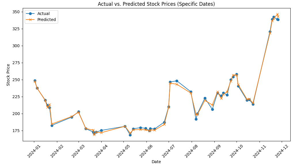
- Prediction for Future Dates: Used the trained model to predict Tesla's stock closing prices for specific future dates in this objective being December 31st 2024.ssary
Technologies Used
- Python
- Scikit-learn
- Pandas
- NumPy
Jupyter Notebook
Data Collection and Processing:
- Loaded historical Tesla stock price data.
- Preprocessed the data by cleaning columns (e.g., removing special characters like $) and converting them into numeric format.
- Checked for and handled missing values to ensure data integrity.
- Visualized historic data based on the values given
import pandas as pd
import matplotlib.pyplot as plt

# Load data
data = pd.read_csv('Tesla_StockPrice_Historical.csv')

# Convert date column to datetime
data['Date'] = pd.to_datetime(data['Date'])

# Sort data by date
data = data.sort_values('Date')

# Check for missing values
print(data.isnull().sum())
Output
Date      0
Close     0
Volume    0
Open      0
High      0
Low       0
dtype: int64
print(data.describe())
Output
                                Date        Volume
count                           1258  1.258000e+03
mean   2022-06-08 09:58:39.872814080  1.264734e+08
min              2019-12-09 00:00:00  2.940168e+07
25%              2021-03-10 06:00:00  7.611178e+07
50%              2022-06-07 12:00:00  1.030910e+08
75%              2023-09-07 18:00:00  1.469126e+08
max              2024-12-06 00:00:00  9.140809e+08
std                              NaN  8.239543e+07
#Format the Date to DateTime
data['Date'] = pd.to_datetime(data['Date'])
# Remove any symbols (like $ or commas) and convert to numeric
data['Close'] = data['Close'].replace('[\$,]', '', regex=True).astype(float)
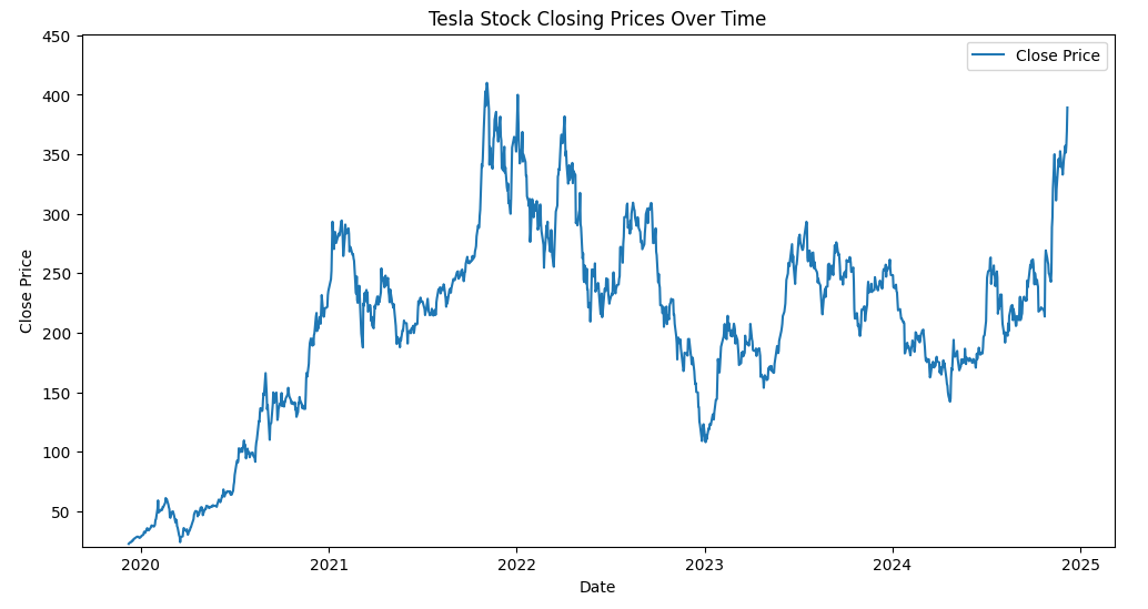
plt.figure(figsize=(12, 6))
plt.plot(data['Date'], data['Close'], label='Close Price')
plt.title('Tesla Stock Closing Prices Over Time')
plt.xlabel('Date')
plt.ylabel('Close Price')
# Set y-axis limits
plt.ylim(data['Close'].min() * 0.9, data['Close'].max() * 1.1) # Adjust the range slightly
plt.legend()
plt.show()
Output
Model Training:
- Created lagging features (Close_t-1, Close_t-2, etc.), moving averages (e.g., 7_day_avg, 30_day_avg), and volatility metrics (e.g., 7_day_volatility) to capture trends and patterns in stock prices.
- Split the dataset into training and testing sets using by splitting.
- Trained a Random Forest Regressor as the predictive model.
- Evaluated the model on the test set using Mean Squared Error (MSE), achieving an MSE of 16.44, which translates to a Root Mean Squared Error (RMSE) of approximately $4.05.
#Addition of Lagging Features


#Add columns for previous days closing prices
data['Close_t-1'] = data['Close'].shift(1)
data['Close_t-2'] = data['Close'].shift(2)

#Calculate Moving Averages to Capture trends
data['7_day_avg'] = data['Close'].rolling(window=7).mean()
data['30_day_avg'] = data['Close'].rolling(window=30).mean()

#Measure Volatility (e.g standard deviation over 7 days)
data['7_day_volatility'] = data['Close'].rolling(window=7).std()

#Measure percent change to track momentum
data['pct_change'] = data['Close'].pct_change()

#Removal of missing values due to moving averages
data = data.dropna()
#Preparing the data for Modelling

#Define X and Y features
X = data[['Open', 'High', 'Low', 'Volume', 'Close_t-1', '7_day_avg', '30_day_avg', '7_day_volatility']]
y = data['Close']

#Train and Test Split
from sklearn.model_selection import train_test_split

X_train, X_test, y_train, y_test = train_test_split(X, y, test_size=0.2, shuffle=False)
print(X[['Open', 'High', 'Low']].head())
Output
         Open     High      Low
1228  $38.13   $39.63   $37.27
1227  $37.62   $38.80   $37.04
1226  $38.04   $38.26   $36.95
1225  $36.13   $37.63   $35.95
1224  $37.90   $38.45   $37.21
# Remove symbols and convert to float
for col in ['Open', 'High', 'Low']:
    X.loc[:, col] = X[col].replace('[\$,]', '', regex=True).astype(float)
#Check for Missing Values: After converting the columns check for any NaN values
print(X.isnull().sum())
Output
Open                0
High                0
Low                 0
Volume              0
Close_t-1           0
7_day_avg           0
30_day_avg          0
7_day_volatility    0
dtype: int64
from sklearn.model_selection import train_test_split

X_train, X_test, y_train, y_test = train_test_split(X, y, test_size=0.2, random_state=42)

from sklearn.ensemble import RandomForestRegressor
from sklearn.metrics import mean_squared_error

model = RandomForestRegressor(n_estimators=100, random_state=42)
model.fit(X_train, y_train)

y_pred = model.predict(X_test)
mse = mean_squared_error(y_test, y_pred)
print(f"Mean Squared Error: {mse}")
Output
Mean Squared Error: 16.441745205325304
MSE represents the average squared error between predicted and actual stock prices. In this case, it’s 16.44 (in squared units,dollars² for stock prices).

Example: Compare the RMSE to the range of the target variable (y). If Tesla’s stock prices range from, say, 300 to 500, then an error of $4.05 may be acceptable.
import matplotlib.pyplot as plt

residuals = y_test - y_pred
plt.figure(figsize=(10, 6))
plt.scatter(y_test, residuals)
plt.axhline(0, color='red', linestyle='--')
plt.xlabel("Actual Values")
plt.ylabel("Residuals")
plt.title("Residual Analysis")
plt.show()
Output�
Feature Importance Analysis
- Evaluated feature importance using the trained Random Forest model to understand which factors contributed most to predictions.
- Identified key features, such as previous day’s closing price (Close_t-1) and moving averages, as the most influential drivers of the model.
importances = model.feature_importances_
features = X.columns
sorted_indices = importances.argsort()

plt.figure(figsize=(10, 6))
plt.barh(features[sorted_indices], importances[sorted_indices])
plt.xlabel('Feature Importance')
plt.title('Feature Importance for Random Forest Model')
plt.show()
Output
# Example feature values for the final prediction
final_features = {
    'Open': 400.0,
    'High': 405.0,
    'Low': 395.0,
    'Volume': 1200000,
    'Close_t-1': 398.0,
    '7_day_avg': 399.5,
    '30_day_avg': 396.0,
    '7_day_volatility': 3.2,
    'Date': '2024-12-31'  # Add the date you wish to predict (datetime)
}

# Convert to a DataFrame
import pandas as pd
final_features_df = pd.DataFrame([final_features])

# Ensure the feature names match those used during training
final_features_df = final_features_df[model.feature_names_in_]

# Make the prediction
final_prediction = model.predict(final_features_df)
print(f"Predicted Closing Price on December 31, 2024: ${final_prediction[0]:.2f}")
Output
Predicted Closing Price on December 31, 2024: $394.25
# Add predictions to a DataFrame for visualization
test_results = X_test.copy()
test_results['Actual'] = y_test.values
test_results['Predicted'] = y_pred
test_results['Date'] = data.loc[y_test.index, 'Date']  # Ensure the Date column matches

# Sort by date for visualization
test_results = test_results.sort_values(by='Date')

# Plot
plt.figure(figsize=(14, 8))
plt.plot(test_results['Date'], test_results['Actual'], label='Actual', marker='o')
plt.plot(test_results['Date'], test_results['Predicted'], label='Predicted', marker='x')
plt.legend()
plt.title('Actual vs. Predicted Stock Prices Over Time')
plt.xlabel('Date')
plt.ylabel('Stock Price')
plt.xticks(rotation=45)
plt.show()
Output
import seaborn as sns

# Plot the distribution of residuals
plt.figure(figsize=(10, 6))
sns.histplot(residuals, kde=True, bins=30)
plt.title('Distribution of Residuals')
plt.xlabel('Residual')
plt.ylabel('Frequency')
plt.show()
Output
# Filter for specific dates
specific_dates = test_results[test_results['Date'].between('2024-01-01', '2024-12-31')]

# Plot
plt.figure(figsize=(12, 6))
plt.plot(specific_dates['Date'], specific_dates['Actual'], label='Actual', marker='o')
plt.plot(specific_dates['Date'], specific_dates['Predicted'], label='Predicted', marker='x')
plt.legend()
plt.title('Actual vs. Predicted Stock Prices (Specific Dates)')
plt.xlabel('Date')
plt.ylabel('Stock Price')
plt.xticks(rotation=45)
plt.show()
Output
On the base + sources:
Tesla Stock Price Prediction